Adaptive and Selective Time-averaging of Auditory Scenes
Richard McWalter & Josh McDermott
Abstract
To overcome variability, estimate scene characteristics, and compress sensory input, perceptual systems pool data into statistical summaries. Despite growing evidence for statistical representations in perception, the underlying mechanisms remain poorly understood. One example of such representations occurs in auditory scenes, where background texture appears to be represented with time-averaged sound statistics. We probed the averaging mechanism using "texture steps" textures containing subtle shifts in stimulus statistics. Although generally imperceptible, steps occurring in the previous several seconds biased texture judgments, indicative of a multi-second averaging window. Listeners seemed unable to willfully extend or restrict this window, but showed signatures of longer integration times for temporally variable textures. In all cases the measured time scales were substantially longer than previously reported integration times in the auditory system. Integration also showed signs of being restricted to sound elements attributed to a common source. The results suggest an integration process that depends on stimulus characteristics, integrating over longer extents when it benefits statistical estimation of variable signals, and selectively integrating stimulus components likely to have a common cause in the world. Our methodology could be naturally extended to examine statistical representations of other types of sensory signals.Sound texture statistics and texture variability.
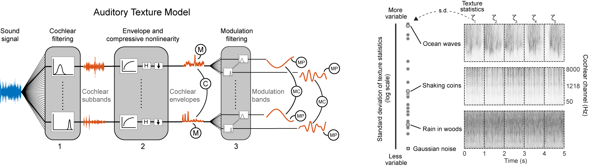
Auditory texture model [McDermott & Simoncelli, 2011] is shown below. Statistics are measured from an auditory model capturing the tuning properties of the peripheral and subcortical auditory system in three stages. The statistics measured from this model include marginal moments and pair-wise correlations at different stages of the model. The subfigure to the right shows the variability of statistics in real-world textures. Left panel shows the standard deviation of texture statistics measured from multiple 1s excerpts of each of a set of 27 textures used in the subsequent experiments. Right panel shows spectrograms of 5 s excerpts of example textures (ocean waves, shaking coins, and rain in the woods). Dashed lines denote borders of 1s segments from which statistics were measured. Some real-world textures have statistics that are quite stable at a time scale of 1s (also evident in the consistency of the visual appearance of 1s spectrogram segments), while others exhibit variability (and would only produce stable estimates at longer time scales).
Audio examples correspond to the texture variability spectrograms (right subplot). In addition to the original texture examples, as displayed in the spectrograms, synthetic textures are provided to demonstrate the realism of the synthesis system for textures with a range of variability. Note, sound interface seems to work best with Firefox of Safari.
| Texture | Original (recorded) | Synthetic |
|---|---|---|
| Waves | ||
| Shaking coins | ||
| Rain in the woods |
Sound texture "step" experiment paradigm.
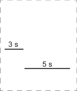
The logic of our main task was to measure the statistics ascribed to one texture stimulus by asking listeners to compare it to another. The stimuli were intended to resemble natural sound textures, and thus varied in a high-dimensional statistical space previously found to enable compelling synthesis of naturalistic textures. To render the discrimination of such high-dimensional stimuli well-posed, we defined a line in the space of statistics between a mean texture stimulus and a reference texture, and generated stimuli from different points along this line (that thus varied in their perceptual similarity to the reference texture). The reference texture was defined by the statistics of a particular real-world texture, and the "mean" texture by the average statistics of 50 real-world textures. On each trial they were asked to judge which of two stimuli was most similar to the reference.
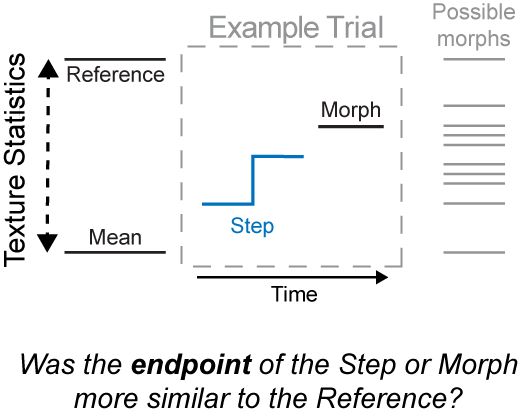
In order to assess the extent over which statistics were averaged by the human auditory system, we asked listeners to compare a texture whose statistics underwent a change mid-way through their duration ("steps") to a texture whose statistics were constant ("morphs"). The idea was that if listeners incorporated the signal preceding the step into their statistic estimate, the estimate would be shifted away from the endpoint statistics, biasing discrimination judgments.
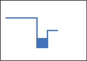
Example spectrograms for step experiment stimuli for the "swamp insects" reference texture. The step occurs 2.5s from the endpoint. The morph examples have statistics from the reference, midpoint and mean.
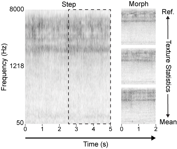
Audio examples correspond to the texture step and morphs (above). The step occurs at 2.5s and moves from 25% to 50% (midpoint) on the statistics continuum. The morphs are at the Reference (top), 50% or midpoint (middle), and mean (bottom).
| Texture Step | Texture Morph | ||
|---|---|---|---|
| Reference | |||
| Note the step location in time is very difficult to detect (see Experiment 1). |
Midpoint | ||
| Mean |
Sound texture morph and step synthesis.
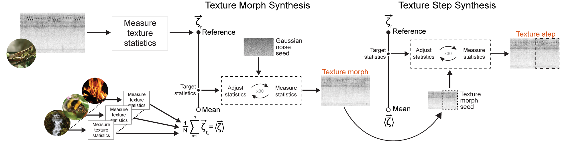
Synthesis of texture morphs and steps. A reference texture was passed to the auditory model, which measured its texture statistics and generated target texture statistics at intermediate points along a line in the space of statistics between the reference texture statistics and the mean statistics of a large set of textures. Synthesis began with Gaussian noise and adjusted the statistics to the target values. Texture steps were created by further adjusting a portion (dashed region) of a texture morph to match the statistics of another point on the line between the reference and mean texture
Experiment 1: Step size selection.
Because it seemed plausible that task performance might be affected by audible changes in the stimulus, we sought to use texture steps that were difficult to detect (but that were otherwise as large as possible, to elicit measurable biases).
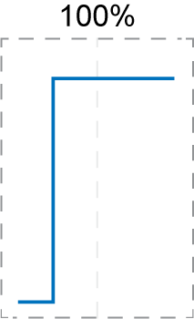
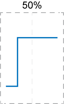
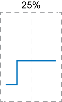
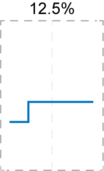
Schematic and Results of Experiment 1 block and trial structure. Listeners heard a texture step and judged whether a change occurred in the first or second half of the stimulus. The step was positioned at either 25% or 75% of the stimulus duration. The right subfigure shows the localization performance of human listeners vs. step size.
Schematic and Results of Experiment 1 block and trial structure. Listeners heard a texture step and judged whether a change occurred in the first or second half of the stimulus. The step was positioned at either 25% or 75% of the stimulus duration. The right subfigure shows the localization performance of human listeners vs. step size.
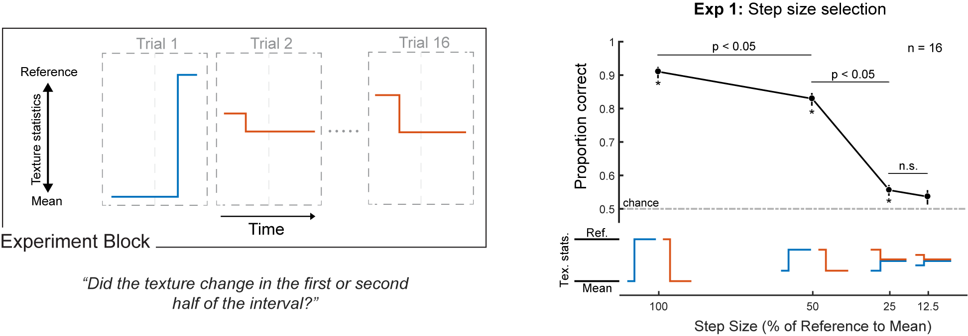
Steps of 25% were difficult to localize, and this step magnitude was selected for use in subsequent step experiments.
Audio examples corresponding to trajectories in Experiment 1 block schematic (left panel). It should be reasonably easy to detect the 100% and 50% steps, but more difficult to detect the 25% and 12.5% steps. First listen to the Reference and Mean, then continue with the 4 examples.
 |
 |
 |
 |
 |
 |
|
|---|---|---|---|---|---|---|
| Sparrows | ||||||
| Swamp insects | ||||||
| Rain |
Experiment 2: Step task validation.
The other requirement of our experimental design was that listeners base their judgment on the end of the step interval. We evaluated compliance with the instructions by comparing discrimination for steps presented at either the beginning or end of the stimulus.
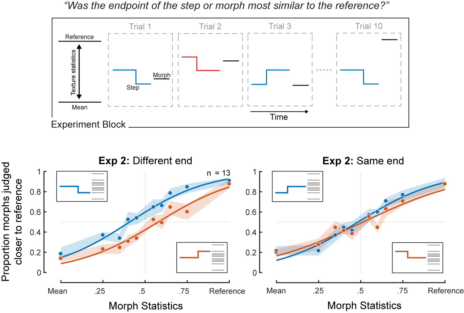
Schematic and Results of Experiment 2 (testing task compliance). Listeners judged whether the step or the morph was most similar to a reference texture. Listeners were informed that the first stimulus (the step) could undergo a change and to base their judgments on the end of that stimulus. Results of Experiment 2 below the experiment block schematic.
Schematic and Results of Experiment 2 (testing task compliance). Listeners judged whether the step or the morph was most similar to a reference texture. Listeners were informed that the first stimulus (the step) could undergo a change and to base their judgments on the end of that stimulus. Results of Experiment 2 below the experiment block schematic.
Audio examples corresponding to trajectories in Experiment 2 block schematic. In this particular block, the trials should get progressively easier. First listen to the Reference and Mean, then continue with the 4 example trials. Again, note the step location in time is difficult to detect.
|
|
 |
 |
 |
 |
|
|---|---|---|---|---|---|---|
| Sparrows | ||||||
| Swamp insects | ||||||
| Rain |
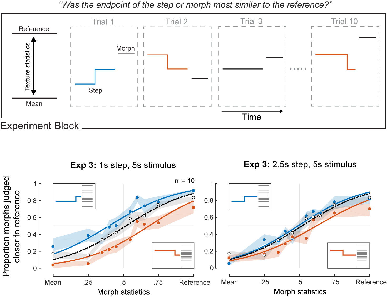
Experiment 3: Effect of stimulus history on texture judgments
Having established that listeners could perform the task, we turned to the main issue of interest: the extent of the stimulus history included in texture judgments. As an initial assay we positioned the step at two different points in time (either 1s or 2.5s from the endpoint and a baseline standard condition with constant statistics at the midpoint).
Schematic and Results of Experiment 3. Listeners judged whether the step or the morph was most similar to a reference texture. Listeners were informed that the first stimulus (the step) could undergo a change and to base their judgments on the end of that stimulus. The results of Experiment 3 are shown below the schematic.
Schematic and Results of Experiment 3. Listeners judged whether the step or the morph was most similar to a reference texture. Listeners were informed that the first stimulus (the step) could undergo a change and to base their judgments on the end of that stimulus. The results of Experiment 3 are shown below the schematic.
Audio examples corresponding to trajectories in Experiment 3 block schematic (above). First listen to the Reference and Mean, then continue with the 4 example trials. Again, note the step location in time is difficult to detect.
|
|
 |
 |
 |
 |
|
|---|---|---|---|---|---|---|
| Sparrows | ||||||
| Swamp insects | ||||||
| Rain |
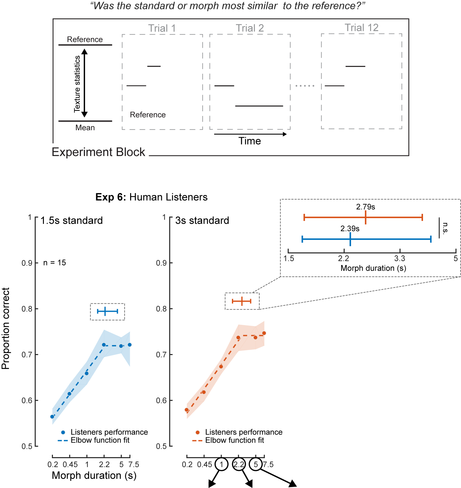
Experiment 6: Constant statistics with varying stimulus duration
To further explore the extent to which integration was obligatory, we investigated whether listeners could instead extend integration when it would benefit performance.
Schematic and Results of Experiment 6. Listeners judged which of two stimuli was most similar to a reference texture. The Standard had constant statistics and duration within blocks; the Morph varied in duration across trials and took on one of two statistic values. Across blocks the Standard took durations of either 1.5 or 3s. The morph varied in duration from 0.2s to 7.5s. Results of Experiment 6 are shown below the schematic.
Schematic and Results of Experiment 6. Listeners judged which of two stimuli was most similar to a reference texture. The Standard had constant statistics and duration within blocks; the Morph varied in duration across trials and took on one of two statistic values. Across blocks the Standard took durations of either 1.5 or 3s. The morph varied in duration from 0.2s to 7.5s. Results of Experiment 6 are shown below the schematic.
Audio examples corresponding to trajectories in Experiment 6 block schematic (above). First listen to the Reference and Mean, then continue with the 3 example trials. The morph will increase in duration for each trial from 1s to 5s.
|
|
 |
 |
 |
|
|---|---|---|---|---|---|
| Sparrows | |||||
| Swamp insects | |||||
| Rain |
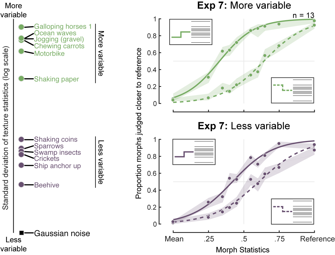
Experiments 7: Effect of texture variability (step discrimination).
Although Experiments 3 and 6 were suggestive of an averaging mechanism whose temporal extent was relatively fixed, there was some reason to think that integration might not always occur over the same time scale. In particular, optimal estimation of statistics should involve a tradeoff between the variability of the estimator (which decreases as the integration window lengthens) and the likelihood that the estimator pools across portions of the signal with distinct statistics (which increases as the integration window lengthens). Because textures vary in their stationarity, the window length at which this tradeoff is optimized should also vary. For highly stationary textures, such as dense rain, a short window might suffice for stable estimates, whereas for less stationary textures, such as the sound of ocean waves, a longer window could be better. We thus explored whether the time scale of integration might vary according to the variability of the sensory signal.
Textures and Results of Experiment 7. Variability in texture statistics measured across 1-s windows for the 12 reference textures from Experiment 7. Variability of Gaussian noise statistics is provided for comparison. Listeners judged whether the endpoint of the step or the morph was most similar to the reference. The step was positioned 2.5s from the endpoint. Results from human listeners, plotted separately for more variable (upper panel) and less variable (lower panel) textures.
Audio examples correspond to the 12 real-world texture recordings used in Experiment 7 and Gaussian noise.
 |
|
|---|---|
| Galloping horses 1 | |
| Ocean waves | |
| Jogging on gravel | |
| Chewing carrots | |
| Motorbike | |
| Shaking paper | |
| Shaking coins | |
| Sparrows | |
| Swamp insects | |
| Crickets | |
| Ship anchor up | |
| Beehive | |
| Gaussian noise |
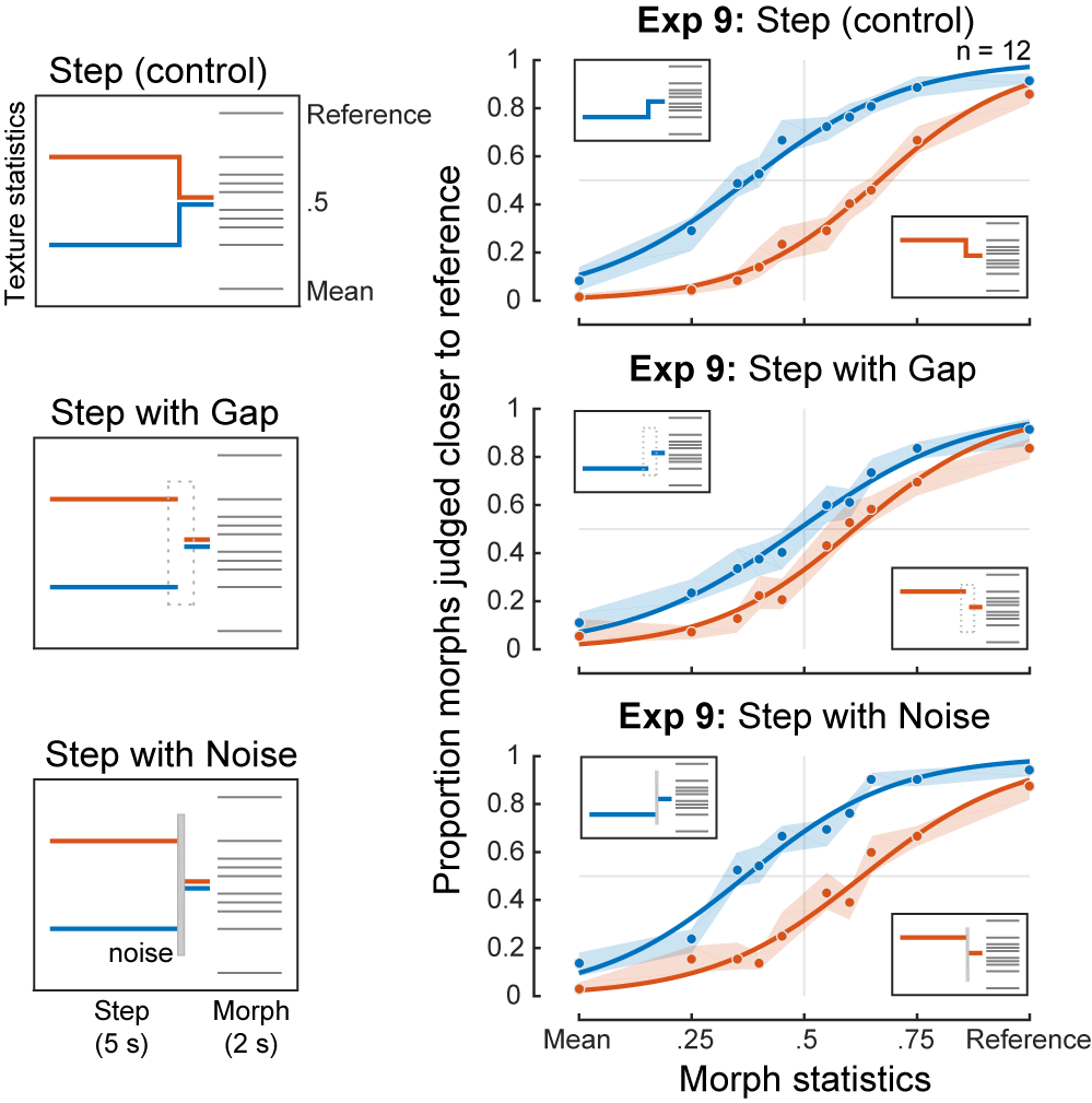
Experiment 9: Effect of noise burst and silent gap.
The apparent presence of an averaging window raised the question of whether the integration process operates blindly over all sound that occurs within the window, or whether integration might be restricted to the parts of the sound signal that are likely to belong to the same texture. We explored this issue by introducing audible discontinuities in the step stimulus immediately following the statistic change.
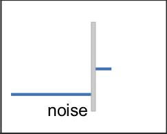
Conditions and Results of Experiment 9. The gap condition included a 200ms silent gap positioned immediately following the step (1s from the endpoint of the step interval). The noise burst condition replaced the gap with a 200ms spectrally matched noise, the intensity of which was set to produce perceptual continuity between the texture before and after it. Listeners judged whether the endpoint of the step or the morph was most similar to the reference. Results for the three conditions are shown in the right subfigure.
Conditions and Results of Experiment 9. The gap condition included a 200ms silent gap positioned immediately following the step (1s from the endpoint of the step interval). The noise burst condition replaced the gap with a 200ms spectrally matched noise, the intensity of which was set to produce perceptual continuity between the texture before and after it. Listeners judged whether the endpoint of the step or the morph was most similar to the reference. Results for the three conditions are shown in the right subfigure.
The audio examples correspond to the conditions of Experiment 9. Only the step interval is presented (5s).
| Step (control) | Step with Gap | Step with Noise | ||||
|---|---|---|---|---|---|---|
 |
 |
 |
 |
 |
 |
|
| Swamp insects | ||||||
| Rain | ||||||
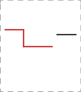
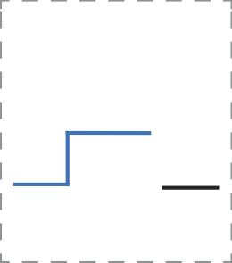
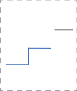
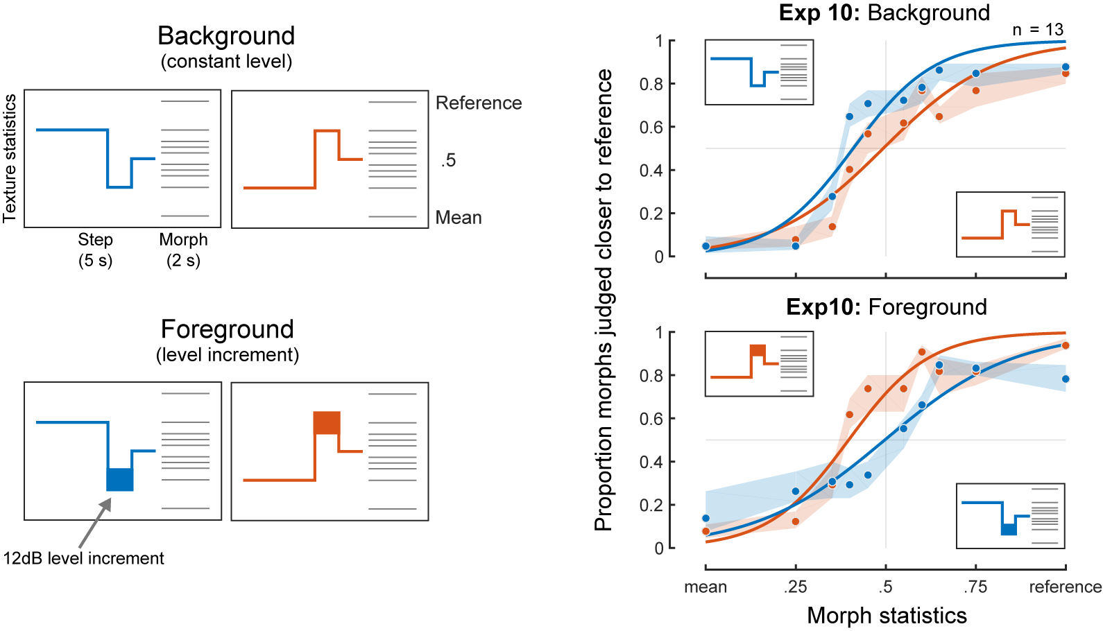
Experiment 10: Exclusion of foreground elements from texture integration.
The finding that integration appears to occur across an intervening noise burst (Experiment 9) raised the question of whether such extraneous sounds are included in the texture integration process.
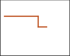
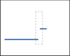
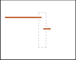
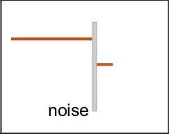
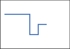
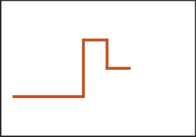
The Background condition was composed of 3 segments with different statistics, creating steps 2s and 1s from the endpoint of the step interval. The grouping of the second segment with the other two was manipulated by increasing the level of the second segment by 12dB (indicated by thicker line in the Foreground schematic). The level increment caused the second segment to be heard as a distinct foreground sound, "behind" which the other segments perceptually completed. Listeners judged whether the endpoint fo the step or the morph was most similar to the reference. Results for Background and Foreground step conditions are shown in the right subfigure. Note that the curves (red and blue) flip when the level increment is included.
The Background condition was composed of 3 segments with different statistics, creating steps 2s and 1s from the endpoint of the step interval. The grouping of the second segment with the other two was manipulated by increasing the level of the second segment by 12dB (indicated by thicker line in the Foreground schematic). The level increment caused the second segment to be heard as a distinct foreground sound, "behind" which the other segments perceptually completed. Listeners judged whether the endpoint fo the step or the morph was most similar to the reference. Results for Background and Foreground step conditions are shown in the right subfigure. Note that the curves (red and blue) flip when the level increment is included.
The audio examples correspond to the schematics on the far right. In each cell the first audio example is the blue step and the second audio example is the red step. Only the step interval is presented (5s).
| Background (constant level) | Foreground (level increment) | |||
|---|---|---|---|---|
 |
 |
 |
 |
|
| Swamp insects | ||||
| Rain | ||||
About the paper
Get the paper here or here (Science Direct).
Email me if you would like the code for the texture morph/step synthesis or the observer model.
Email me if you would like the code for the texture morph/step synthesis or the observer model.