Figure 1
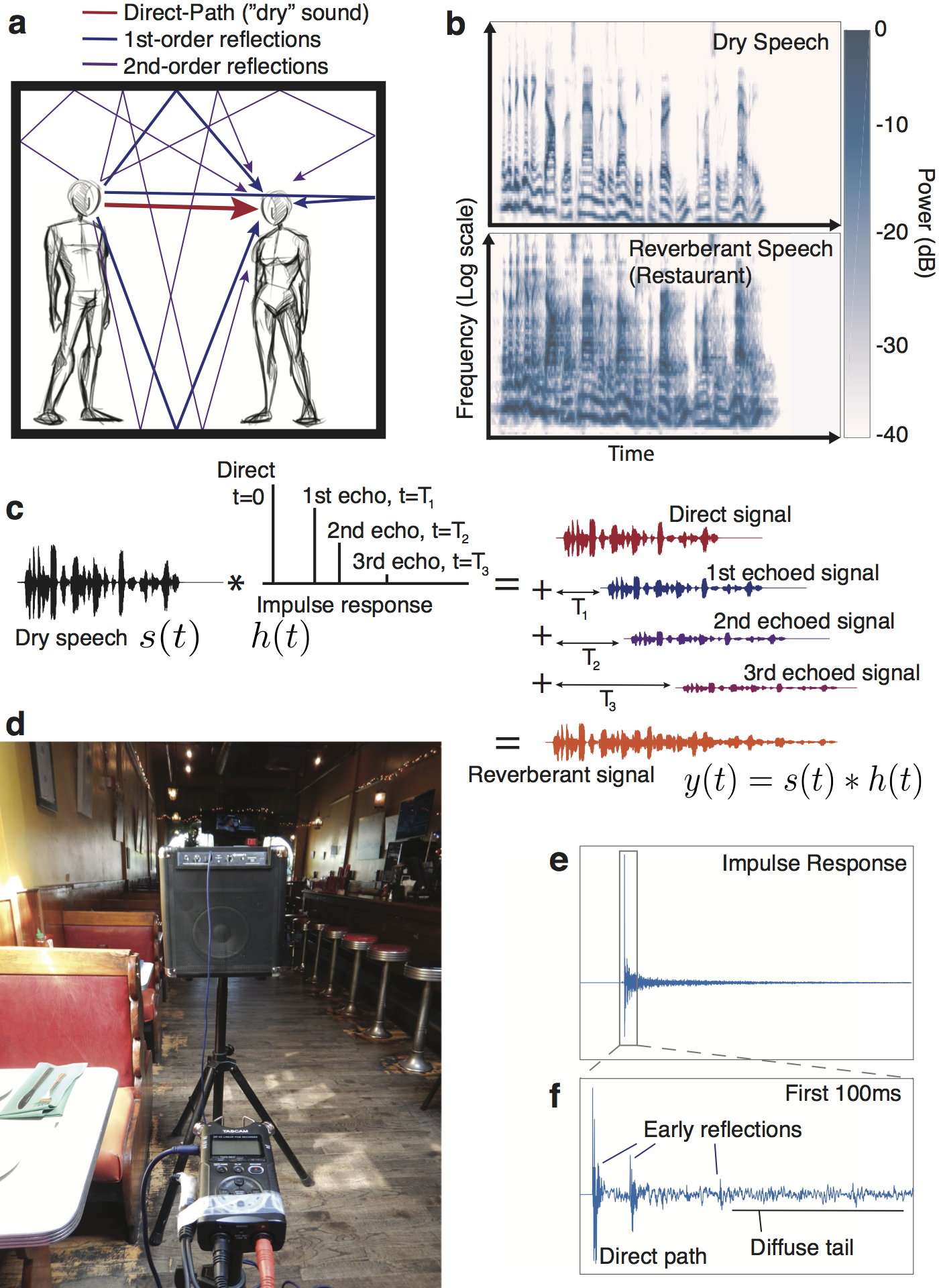
Figure 1. The effect of reverberation. A. Sound reaches a listener directly as well as via reflections off surrounding surfaces. B. Reverberation distorts the structure of source signals, shown by cochleagrams (representations of the spectrotemporal structure of sound as it is believed to be encoded by the auditory periphery) of speech without (top) and with (bottom) reverberation. C. The effect of reverberation on a sound is described mathematically by the convolution of the sound with the impulse response (IR) of the environment, . The original sound is repeated, time-shifted and scaled for every non-zero point in the IR and the resulting signals are summed. This process is illustrated for a schematic IR with 3 echoes. For clarity these echoes are more widely spaced than in a naturally occurring IR. D. A photograph of the apparatus we used to measure IRs -- a battery powered speaker and a portable digital recorder in one of the survey sites, a restaurant in Cambridge, Massachusetts. E. An IR measured in the room shown in (D). Every peak corresponds to a possible propagation path; the time of the peak indicates how long it takes the reflected sound to arrive at the ear and the amplitude of the peak the amplitude of the reflection, relative to that of the sound that travels directly to the ear. F. The first 100ms of the IR in (E). Discrete early reflections (likely 1st or 2nd order reflections) are typically evident in the early section of an IR, after which the reflections become densely packed in time, comprising the diffuse tail.
Figure 2
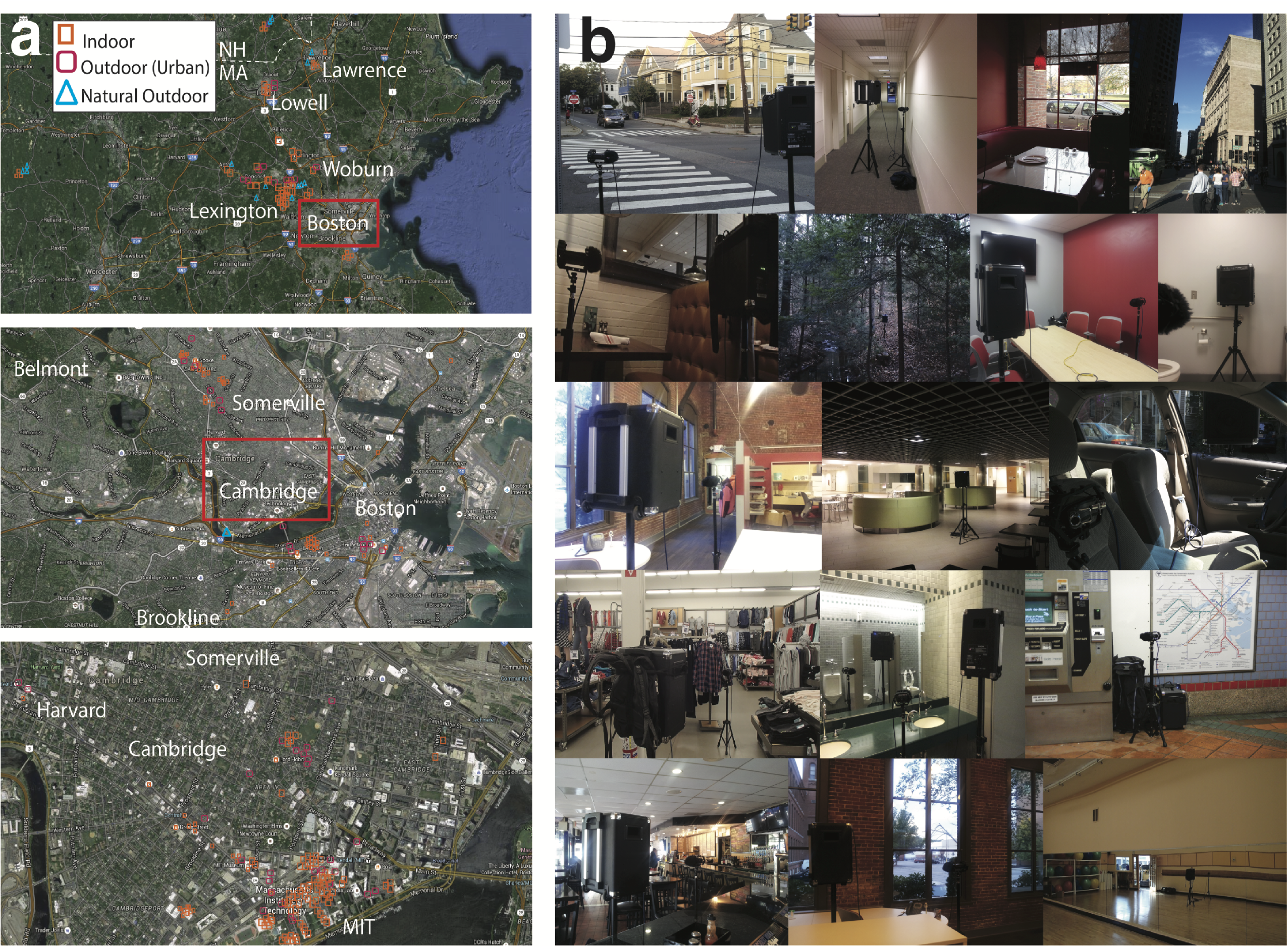
Figure 2. Survey of natural reverberation. A. Maps showing the location of the 271 measured survey sites. Top: Massachusetts and New Hampshire; Center: Greater Boston area with most survey sites in Boston, Cambridge and Somerville; Right: Cambridge, the location of most survey sites. Red boxes indicate the region shown in higher detail below. B. Photographs of 14 example locations from the survey (from top-left: suburban street corner, hallway, restaurant, Boston street, restaurant booth, forest, conference room, bathroom, open plan office, MIT building 46, car, department store, bathroom, subway station, bar, office, aerobics gym).
Figure 3
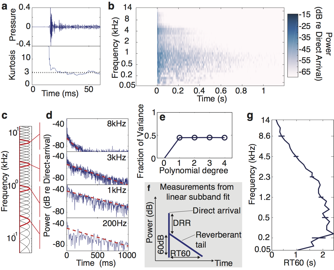
Figure 3. Measurement and analysis of reverberation. A. The first 60ms of the restaurant IR from Figure 1 (top) with the kurtosis (bottom) computed over a 10ms sliding window. The dotted line shows the kurtosis of Gaussian noise. Apart from the very earliest section, the IR is well described by Gaussian statistics. B. Cochleagram of the restaurant impulse response from Figure 1D—F). C. Transfer functions of simulated cochlear filters used for subband analysis. Filters in red are those corresponding to the subbands shown in D. D. Power in frequency subbands of the impulse response, showing how it redistributes energy in particular frequency bands over time. Dashed lines show best-fitting exponential decay. E. Fraction of variance of subband log-power accounted for by polynomials of varying degree. A degree of 1 corresponds to exponential decay, while a degree of 0 corresponds to fitting to the mean. F. Schematic of reverberation measurements made using linear fits to frequency channel log-power: the Reverberation Time to 60dB (RT60) is the time taken for the reverberation to decay 60dB; the Direct-to-Reverberant Ratio (DRR) is the difference in power between the direct arriving sound and the initial reverberation. G. Measured RT60 (i.e. decay rate) from each subband of the example IR in (A). Errorbars show 95% confidence intervals obtained by bootstrap.
Figure 4
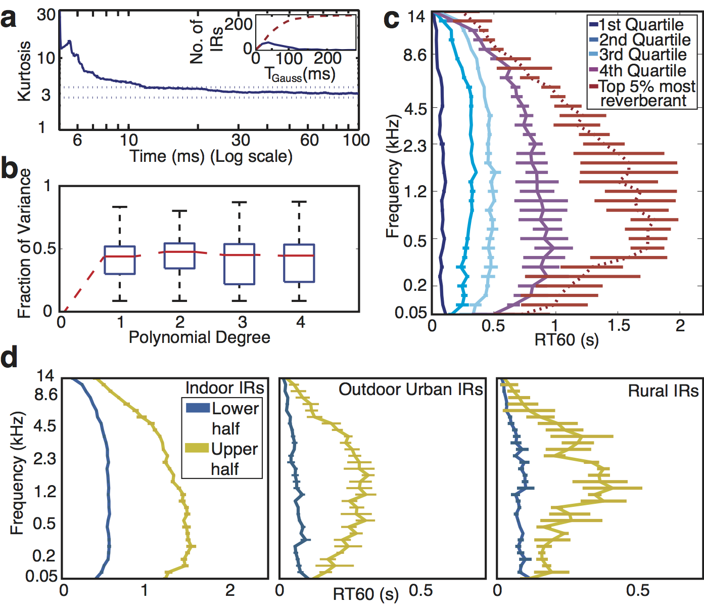
Figure 4. Statistics of natural reverberation A. IRs have locally Gaussian statistics. Median kurtosis (sparsity) vs. time for the surveyed IRs. The kurtosis for each IR was calculated in 10ms windows; the line plots the median across all surveyed IRs for each time point. Here and elsewhere in this figure, errorbars show 95% confidence intervals obtained by bootstrap. Horizontal dotted lines show 95% confidence intervals of the kurtosis of 10 ms Gaussian noise excerpts. Inset: histogram (solid line) of the time at which the IR kurtosis reached the value for Gaussian noise (T_Gauss) across the surveyed IRs, along with the corresponding cumulative distribution function (dashed line). B. Energy decays exponentially. Box-plots of the distribution of the Fraction of Variance of IR subbands accounted for by polynomial decay models of degree P for P=[1,2,3,4]. The model was fit to the data recorded by the left channel of the recorder and evaluated on the data recorded by the right channel (i.e. the variance explained was computed from from the right channel). The two channels were connected to different microphones that were oriented 90 degrees apart. They thus had a different orientation within the environment being recorded, and the fine structure of the recorded IRs thus differed across channels. Using one channel to fit the model and the other to test the fit helped to avoid overfitting biases in the variance explained by each polynomial. C. Frequency dependence of reverberation time (RT60) in the surveyed IRs. Lines plot the median RT60 of quartiles of the surveyed IRs, determined by average RT60. Dotted red line plots the median value for the most reverberant IRs (top 5%). D. Median RT60 profiles (as in C except using halves rather than quartiles because of smaller sample sizes) for indoor environments (N = 269), outdoor urban environments (e.g. street corners, parking lots, etc., N = 62) and outdoor rural environments (forests, fields, etc., N = 29). To increase sample sizes we supplemented the 271 IRs measured here with those of two other studies (Jeub et al., 2009; Warren ).
Figure 5
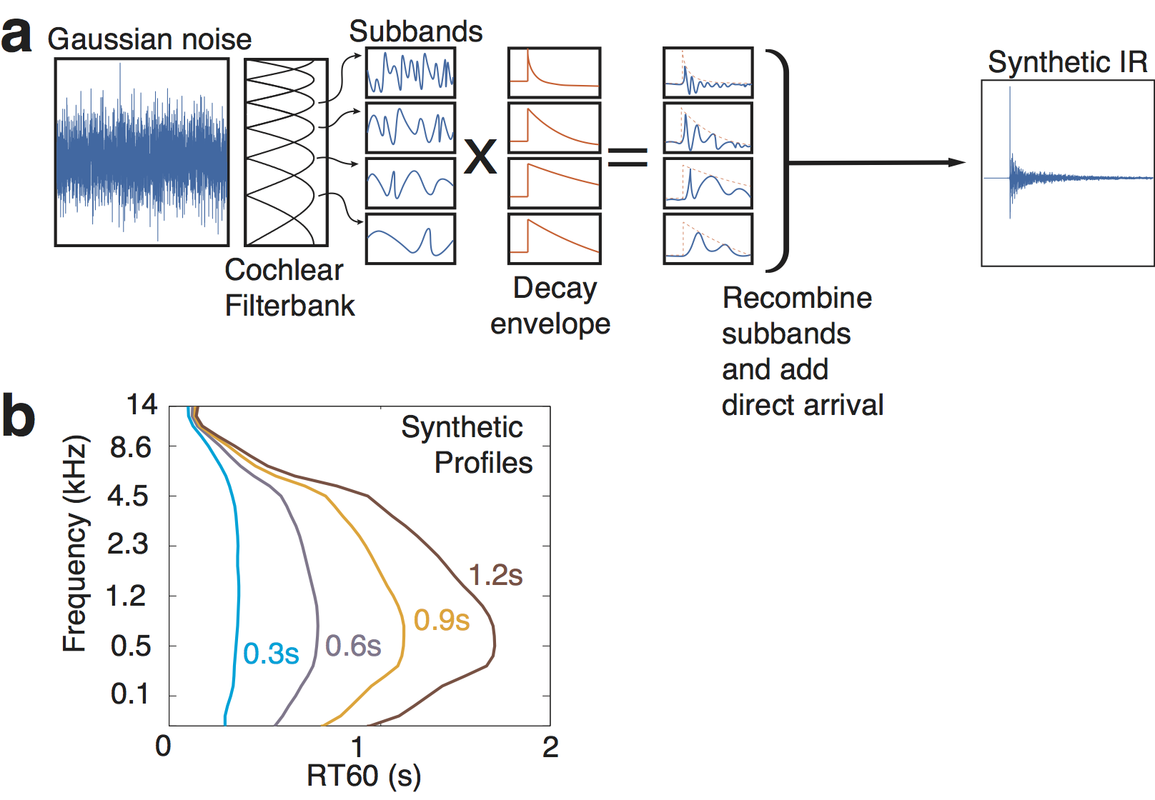
Figure 5. Synthetic IR generation. A. IRs were generated by filtering Gaussian noise into cochlear subbands and multiplying each subband by an amplitude envelope. The modified subbands were then recombined to yield a broadband synthetic IR. The temporal form of the decaying envelopes and the frequency dependence of decay rates were manipulated to produce IRs that were either consistent with the statistics of real-world IRs or that deviated from them in some respect. B. Synthetic decay rate profiles were computed that shared the variation in frequency, and the variation of decay-rate-profile with average RT60, with the surveyed IR distribution (Figure 4C).
Figure 6
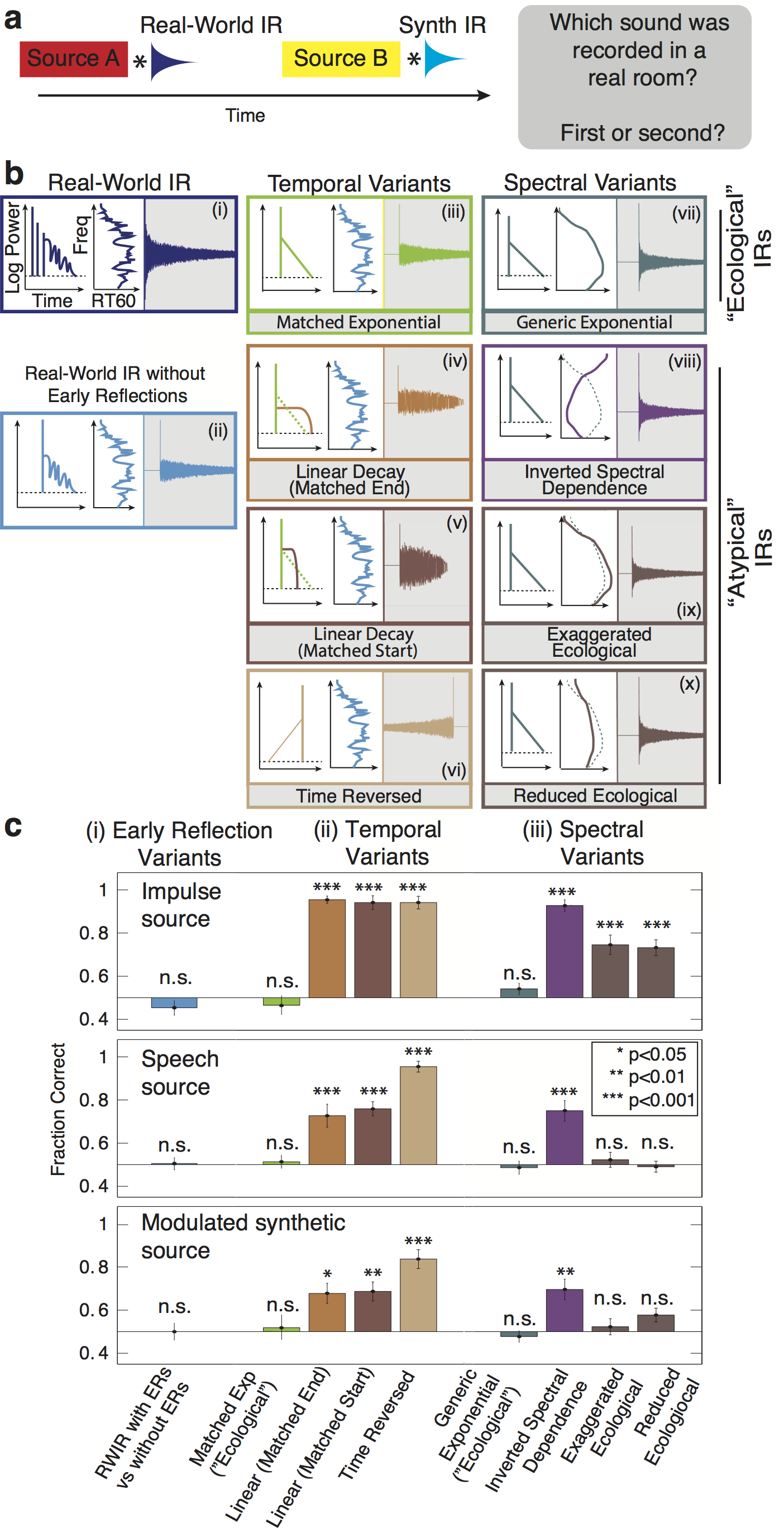
Figure 6. Discrimination of synthetic reverberation (Experiment 1). A. Schematic of trial structure. Two sounds were played in succession, separated by a silent interval. Each sound was generated by convolving a source signal (an impulse, a spoken sentence, or a modulated noise) with an impulse response. The impulse response was a real-world IR for one sound and one of the synthetic variants for the other (matched in RT60). Listeners judged which of the two sounds was recorded in a real room. B. IR variants used in psychophysical experiments, varying in the presence of early reflections (i--ii), temporal decay (iii--vi), and spectral dependence of decay (vii--x): (i) Real-world IR; (ii) Real-world IR with the early reflections removed; (iii) synthetic exponential decay with RT60 and DRR profiles matched to a real-world IR; (iv--v) synthetic linear decay matched to a real-world IR in starting amplitude or audible length (vi) time-reversed exponential decay; (vii) synthetic exponential decay with RT60 and DRR profiles interpolated from the real-world IR distribution; (viii--x) inverted, exaggerated, or reduced spectral dependence of RT60. C. Task performance (proportion correct) as a function of the synthetic IR class for three source types: impulses (top; yielding the IRs themselves), speech (middle) and modulated noise (bottom). Errorbars denote standard error of the means. Asterisks denote significance of difference between each condition and chance performance * p<0.05, ** p<0.01 and *** p<0.001; two-sided t-test).
Figure 7
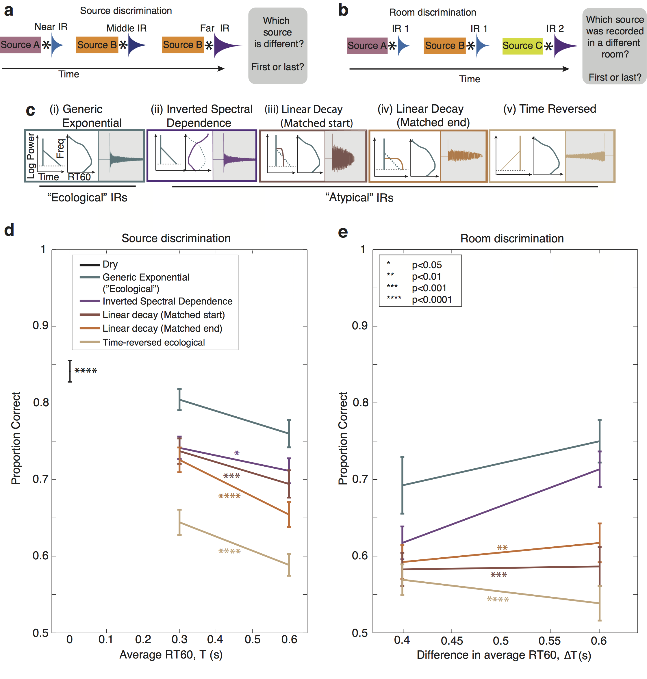
Figure 7. Perceptual separation of source and IR (Experiments 2 and 3). A. Schematic of trial structure for Experiment 2 (discrimination of sources in reverberation). Three sounds were played in succession, separated by silent intervals. Each sound was generated by convolving a source signal (modulated noise) with a different impulse response. The impulse responses were all a particular type of synthetic variant, and had the same RT60 but differed in DRR (simulating different distances of the source from the listener). Listeners judged which of the three sources was different from the other two. B. Schematic of trial structure for Experiment 3 (discrimination of IRs in reverberant sound). Three sounds were played in succession, separated by silent intervals. Each sound was generated by convolving a source signal (modulated noise) with an impulse response. The impulse responses were all a particular type of synthetic variant. Two of them were identical and the third had a longer RT60 (simulating a larger room). Listeners judged which of the three sources was recorded in a different room. C. IR variants used to probe the effect of reverberation characteristics on perceptual separation. All IRs introduced equivalent distortion in the cochleagram. D. Source discrimination performance (proportion correct) as a function of IR decay time for different synthetic IR classes. Errorbars denote standard error of the means. Asterisks denote significance of difference between average performance in each condition and that of the Generic Exponential condition. E. IR discrimination performance (proportion correct) as a function of the IR decay time for different synthetic IR classes.
Figure S1
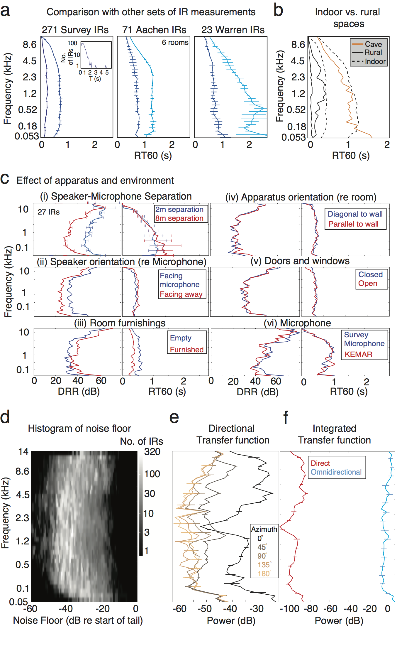
Figure S1. Impulse Response Measurements. A. Comparison between our surveyed IRs (left) and two other sets of IRs: a set measured for the evaluation of dereverberation algorithms (Jeaub et al., 2009) (center) and a set measured for musical use (right; measured by Chris Warren ). All panels plot the median subband RT60 (median taken across the upper and lower halves of a data set), as in Figure 4D. Errorbars (here and throughout this figure) show 95% confidence intervals obtained by bootstrap. The other two sets contain longer IRs, but show qualitatively similar frequency dependence of RT60 to that observed in our data set. Inset in left panel shows a histogram of the median subband RT60s across the surveyed IRs. B. Comparison between the decay rates in an example IR from a cave with those from the indoor and rural IRs from Figure 4D. Indoor and rural IRs are subdivided into more and less reverberant halves, as in S1A. The cave IR (measured by Chris Warren ) shows the same qualitative form as very reverberant indoor spaces. C. Effect of apparatus and environment on IR properties. The DRR and RT60 are plotted for comparison measurements made in a single room with either the apparatus or the room altered between measurements. Altering the (i) speaker-microphone distance or (ii) speaker orientation affects the DRR but only very slightly effects the RT60. Furnishing a room (iii) reduces both the DRR and RT60 relative to the empty room. Neither (iv) rotating the apparatus within the room (v), opening doors and windows, nor (vi) changing the microphone appreciably affected DRR or RT60. D. Histogram of the noise floors of our IR measurements, measured in each subband relative to the subband DRR. The variation is due to the variation in background noise at the survey sites. E. The transfer function of our speaker and microphone were measured in an anechoic chamber with the microphone located 2m from the speaker at varying azimuths relative to the speaker face (the microphone always faced the speaker). Each measurement was made by broadcasting the 3-minute survey Golay sequence (which has a flat spectrum) and plotting the spectrum of the recorded broadcast. F. Total speaker transfer function. The directional transfer functions in (E) were interpolated to approximate a spherical directional spectrum of the speaker and this was integrated over azimuth to estimate the ominidirectional transfer function (blue), which contains the spectral contribution illuminating the environment. This is compared with the spectrum of the signal emanating directly from the speaker face (red). We assume the energy contributing to the IR tail is filtered by the omnidirectional transfer function while the direct arrival is filtered by the direct transfer function and when we compute DRR values from the measured IRs we account for this frequency variation (see Methods).
Figure S2
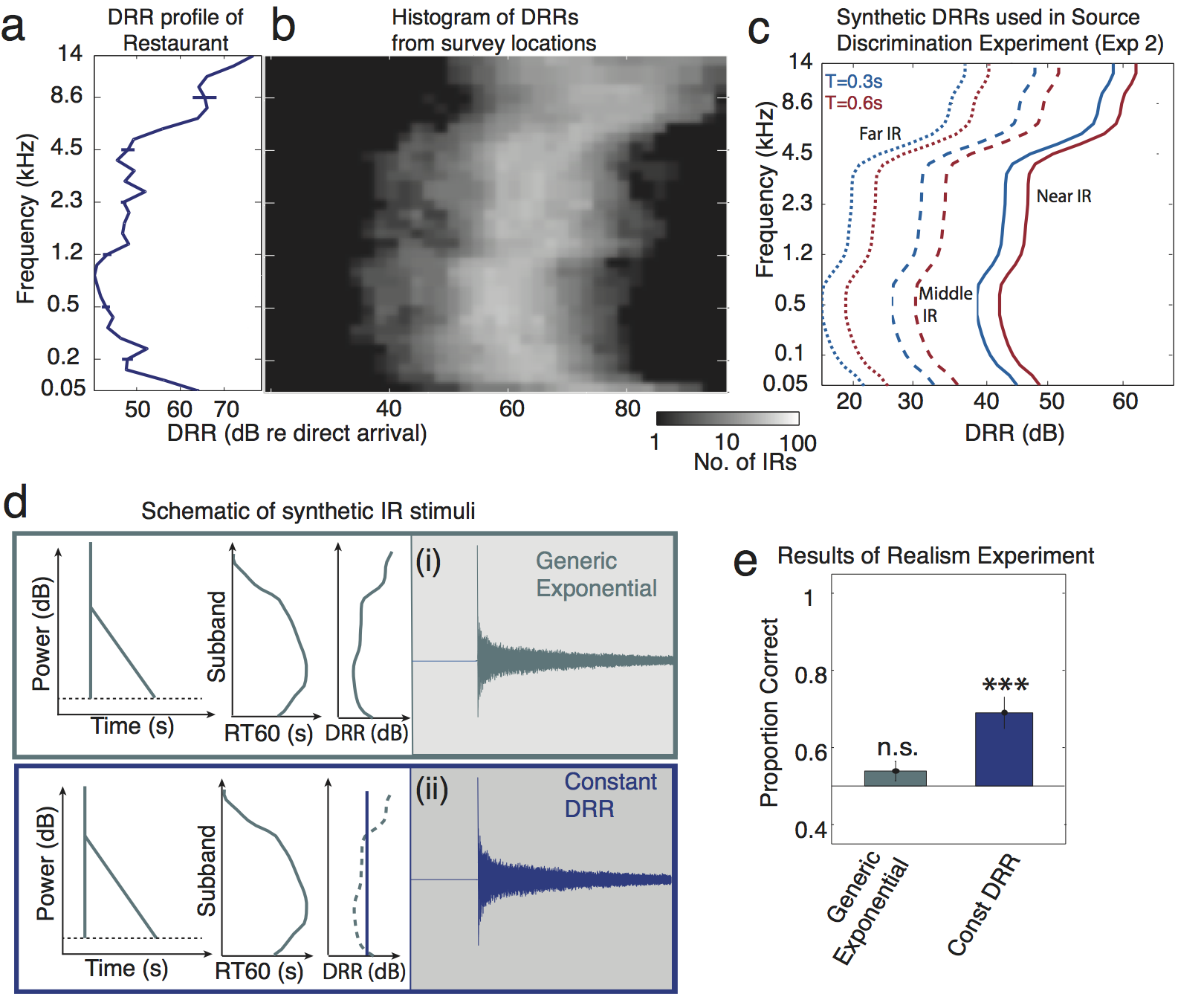
Figure S2. Direct-to-Reverberant Ratio (DRR) -- Measurements and Experiments. A. The DRR profile of the example IR from Figures 1 and 3. See Figure 3F for schematic of DRR measurement. Errorbars show 95% confidence intervals obtained by bootstrapping from the acoustic measurement (by fitting the exponential decay model to multiple random subsets of samples from the time series). B. Histogram of subband DRRs of all surveyed IR locations. C. DRR profiles used to create synthetic IRs in the source discrimination experiment (Experiment 2). We observed a weak dependence of median DRR on broadband RT60; to mimic this effect in our synthetic IRs the long experimental IRs (T=0.6s) had slightly lower DRRs than the short experimental IRs (T=0.3s). D. Conditions from Experiment 1 (real vs. synthetic reverberation discrimination) in which DRR was manipulated. Listeners discriminated Generic Exponential IRs and IRs with constant DRR (in which the DRR was set to the mean value of the Generic Exponential IR DRR across subbands) from real-world IRs. E. The proportion of trials in which human subjects correctly identified the synthetic IR for each IR type. The Generic Exponential data is replotted from Figure 6. Asterisks denotes p<0.001 (two-tailed t-test) as in Figure 6.
Figure S3
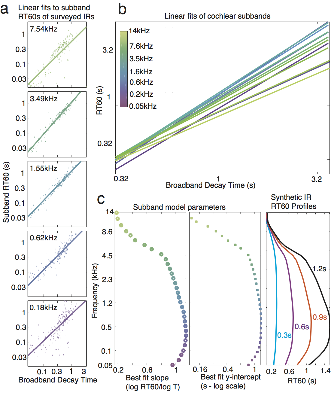
Figure S3. Generation of generic exponential synthetic IR parameters. A. The measured RT60 of each surveyed IR are plotted (dots) for example subbands as a function of the broadband IR RT60 (i.e. the length of the IR). For each subband a line was fitted and used to calculate RT60 values for a given frequency and broadband RT60. B. Linear fits from all cochlear subbands, showing that RT60s in different frequency subbands scale differently with broadband RT60, producing variation in the degree of frequency dependence of decay. C. The fitted parameters of slope (left) and y-intercept (center) for each subband are plotted along with example synthetic IR profiles generated from the fits (right).
Figure S4
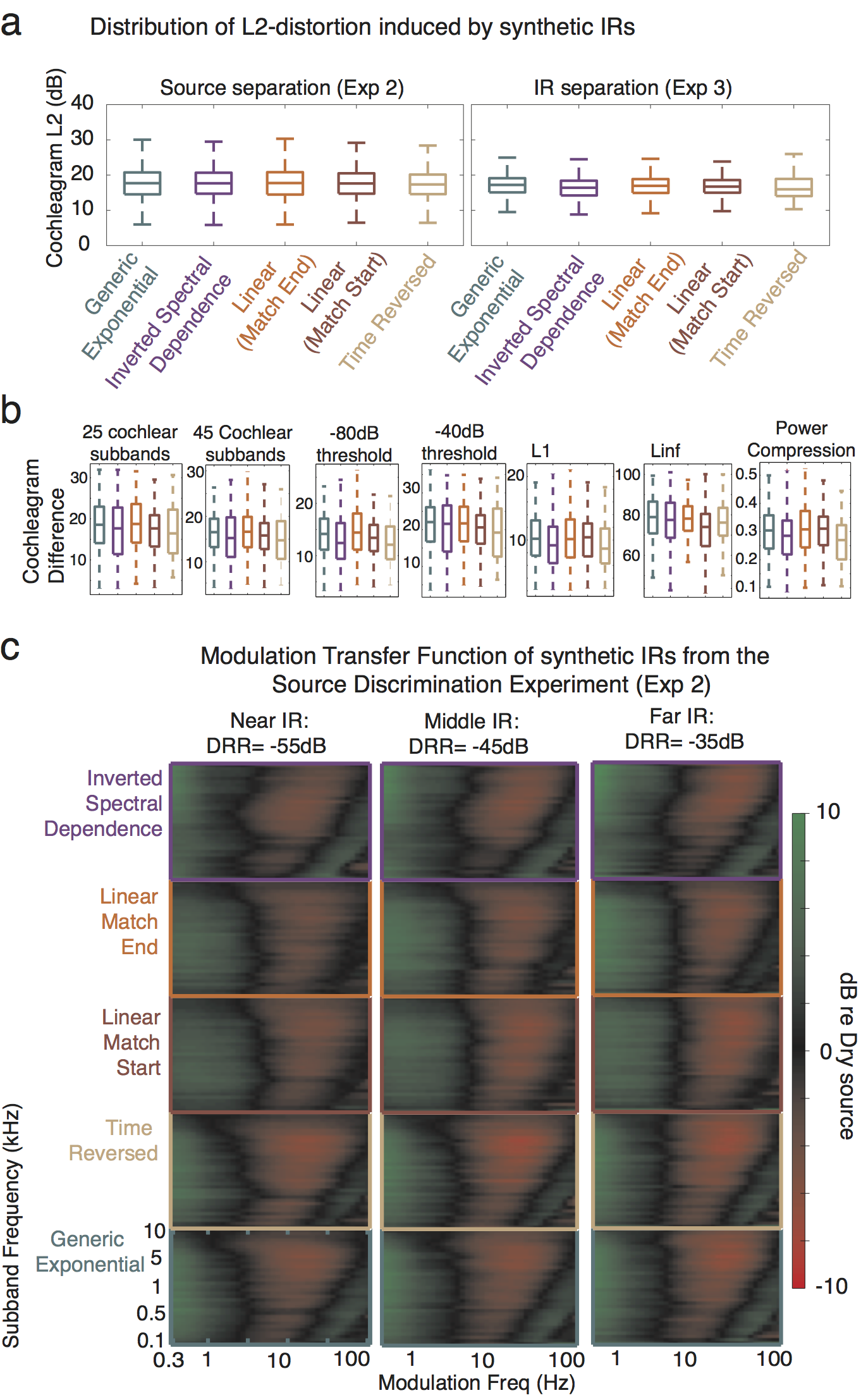
Figure S4. Signal distortion of synthetic IRs. A. Box-plots of the distribution of MSE-distortion introduced by synthetic IRs to the stimuli used in the source discrimination (Exp 2; left) and IR discrimination (Exp 3; right) experiments. The box outlines the 25th, 50th and 75th percentiles. The whiskers delineate the minimum and maximum distortion values. B. MSE distortion is robust to computational details of the cochleagram. Box-plots show the distribution of MSE distortion in the cochleagram across the different IR types (as in S4A) for a range of changes to the cochleagram, from left-to-right: fewer subbands, more subbands, lower threshold, higher threshold, L1-norm (rather than L2), L-infinity norm, exponential compression () rather than logarithmic. C. Modulation Transfer Functions for the synthetic IRs used in Experiment 2. These were obtained by subtracting the modulation spectrum of the dry source signal from that of the corresponding reverberant stimulus presented on an experimental trial, and then averaging this difference over all stimuli. The dry and reverberant signals were first normalized to have the same RMS level and hence the transfer function is symmetric around 0dB.
Figure S5
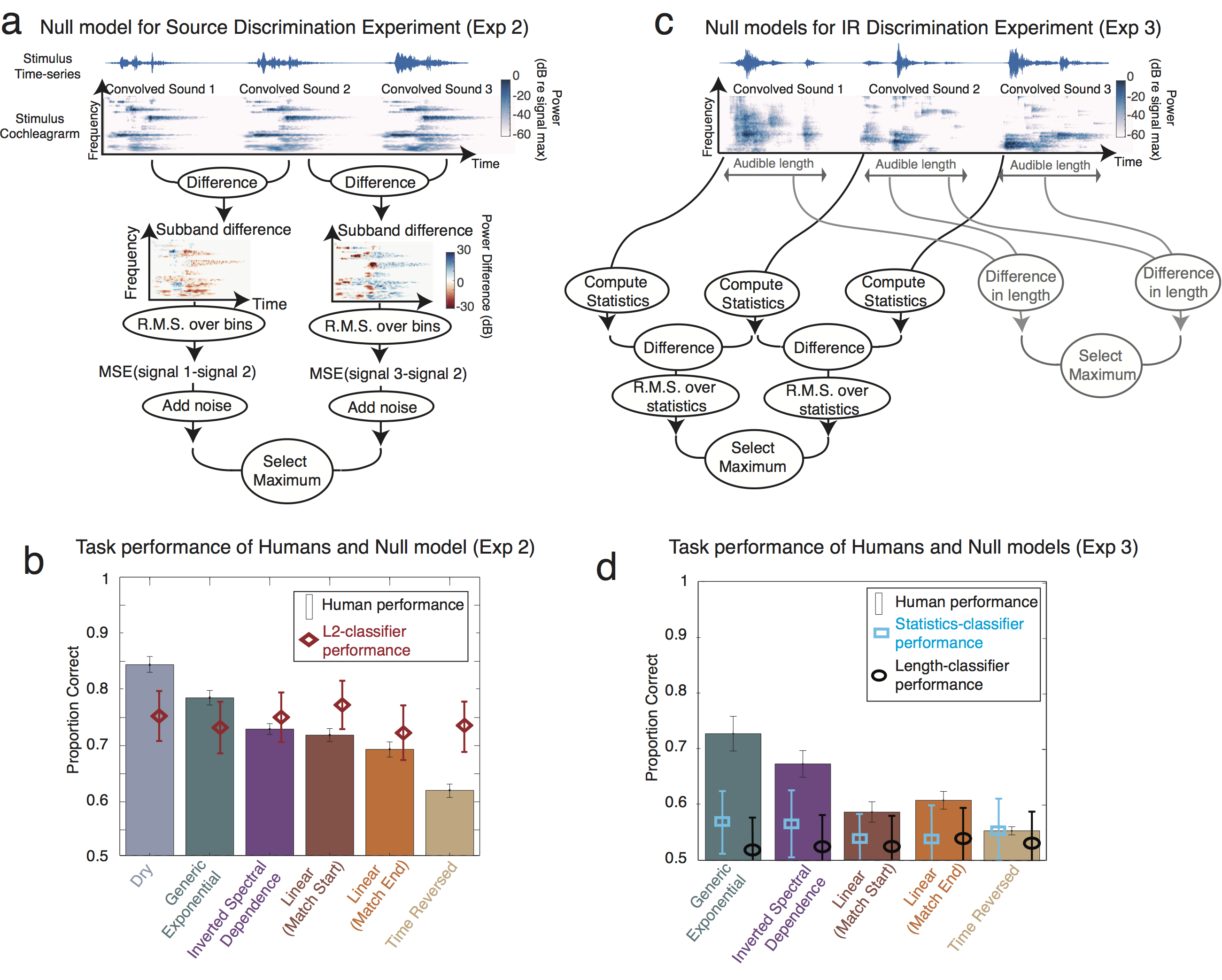
Figure S5. Null models of separation task performance. A. Schematic of the Null Model for source discrimination using cochleagram differences. B. Human performance on the source discrimination experiment compared with the null model. Results from IRs of differing length (Figure 7B) have been averaged. Error bars show 95% confidence intervals obtained by bootstrap. Random noise was added to the decision stage of the null model to equate average performance across all IR classes with that of humans. C. Schematic of two null models for IR discrimination using either cochleagram statistics or audible signal length. D. Human performance on the IR discrimination experiment compared with the null models. Results from IRs of differing length (Figure 7D) have been averaged. Error bars of both human and null model performance show 95% confidence intervals obtained by bootstrap.