Priors and likelihood (Figure 3)
Click the cochleagrams in the figures to hear the corresponding sound.
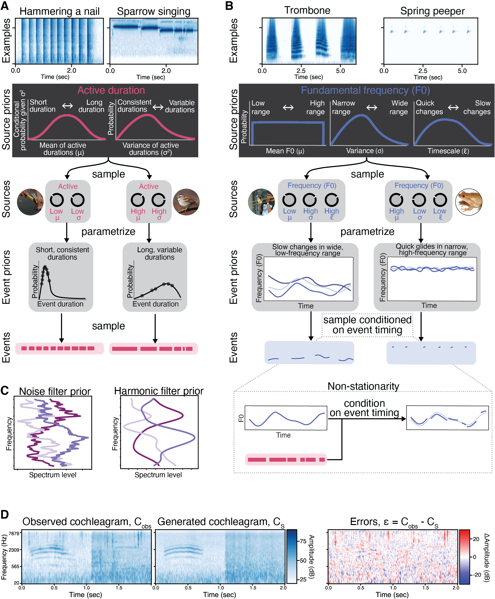
Prior and likelihood, illustrated with recorded natural sound examples. A) Hierarchical priors on event duration. Hammering nails results in short, consistent impacts, while the song of a white-throated sparrow comprises longer tones of variable duration. To capture such regularities, we use a hierarchical model. For each source, the source parameters μ (mean duration) and σ2 (variance) are sampled from the source priors (a normal-inverse-gamma distribution). The source parameters define the event priors (log-normal distributions) from which the event durations are sampled. Different source parameters capture different regularities: the hammer impacts can be modeled with a low mean and low variance, while the sparrow song requires a high mean and high variance. B) Hierarchical priors on fundamental frequency. The trombone's fundamental frequency is in a low, wide frequency range, and changes slowly, while the spring peeper is in a high frequency range and changes quickly by a small amount. For each source, the source parameters μ (mean), σ (kernel variance) and ℓ (kernel lengthscale) are source parameters that are sampled from source priors. These source parameters define the Gaussian process event priors from which event fundamental frequency trajectories are sampled. Different source parameters capture different regularities: the trombone can be captured by low mean, high variance, and high lengthscale, while the spring peeper can be captured by high mean, low variance, and low lengthscale. We depict the Gaussian process priors by showing samples of potential trajectories. To account for the possibility that excitation trajectories might change in their properties from event to event (e.g., a dog panting creates different amplitudes on the in- and out-breath), we used a non-stationary Gaussian process kernel (see Supplmentary Figure 1 for more detail). This required the Gaussian process event priors to be conditioned on the timing of events. C) Prior over filter shape. We used different priors for the filters of different sound types, so that the spectra of harmonic sources tended to be smoother than those of noise sources. This difference was implemented with a Ornstein-Uhlenbeck kernel for noises and a squared-exponential kernel for harmonics. We depict the Gaussian process priors by showing samples. D) To calculate the likelihood, the observed and generated cochleagrams are compared under a Gaussian noise model.
Attributions
Sounds
- inspectorj (hammering nails close, source: Freesound, license CCBY4.0)
- phonosupf (trombone glissandi, source: Freesound, license: CC0)
- Mdf (spring peeper, source: Wikipedia, license: CC BY-SA 3.0)
Images
- robbiesaurus (trombone player, source: Wikimedia, license: CC BY-SA 2.0)
- brian.gratwicke (spring peeper, source: Wikimedia, license: CC BY 2.0)
- Fæ (hammering, source: Wikimedia, public domain)
- Cephas (sparrow singing, source: Wikimedia, license: CC BY-SA 3.0)